Most books on the subject of numerical method for approximating solutions of ODEs agree that the region of absolute stability of a method is one of the most important factors determining its performance when applied to different classes of problems. But, surprisingly, there are discrepancies in how that region is defined!
While some definitions are mutually equivalent, they generally fall into two classes that are inequivalent in that, for some well-known methods, using one class of definitions the region is empty while using the other it is non-empty. Below we provide the definitions from eight well-known books on the subject, with four of the definitions belonging to one camp, and four to the other. The basic dichotomy that distinguishes the two groups is whether they require perturbations of numerical solutions of the linearized model problem y' = λ y with step size h to tend to zero as the number of steps goes to infinity (Atkinson, Burden-Faires, Conte-DeBoor, Iserles), or only to remain bounded (Butcher, Dahlquist, Gear, Leveque).
Of course the distinction is largely a matter of convention. We could call the stronger condition (decay to zero) `absolute stability', and the weaker condition (boundedness) `weak' absolute stability. Or we could call the weaker condition `absolute stability' and the stronger one `strong absolute stability'. If the definition that requires decay to zero is used, the region of absolute stability of both the Leapfrog and Milne-Simpson methods is empty, while if the definition that requires boundedness is used, the region of absolute stability of the Leapfrog method is the interval (-i, i) on the imaginary axis, and the region of absolute stability of the Milne-Simpson method is the origin. The non-empty regions of these two methods and the regions of other methods based on the same definition seem more informative in explaining the behavior of those methods. Using that definition, the property of 0-stability that is required for a method to be convergent corresponds to the origin being in its region of absolute stability. This is not the case for the definition requiring decay to zero, as the two convergent examples mentioned above demonstrate. Finally, the definition requiring only boundedness makes it more compatible with the behavior of both of the two most important classes of PDEs exhibiting well-posed Cauchy problems, the parabolic and the hyperbolic. It is for these reasons that we have followed this convention in our treatment as well. We will group the examples below according to this division, with the ones requiring boundedness first, followed by the ones requiring decay to zero.
The references that we cite are:
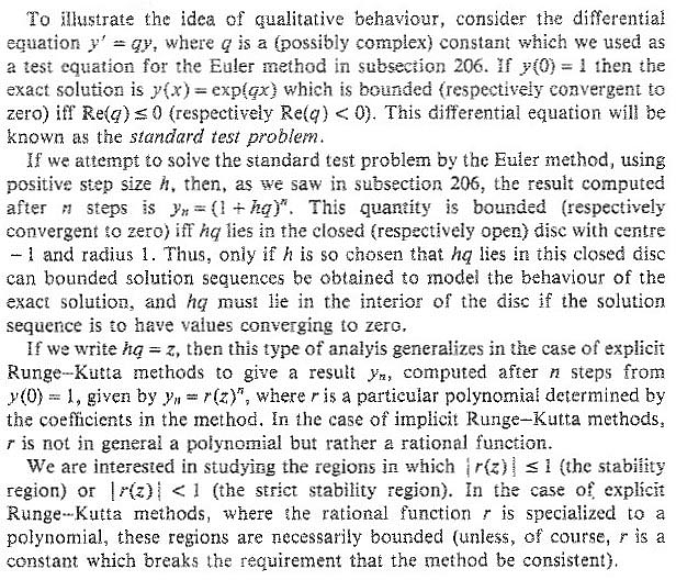
This differential equation [y'=qy] will be known as the standard test problem...If we write hq=z ... We are interested in studying the regions in which |r(z)| ≤1 (the stability region) or |r(z)|<1 (the strict stability region)
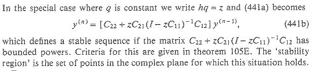
In the special case where q is constant we write hq=z and (441a) becomes ... which defines a stable sequcnce if the matrix ... has bounded powers. The `stability region' is the set of points in the complex plane for which this situation holds.
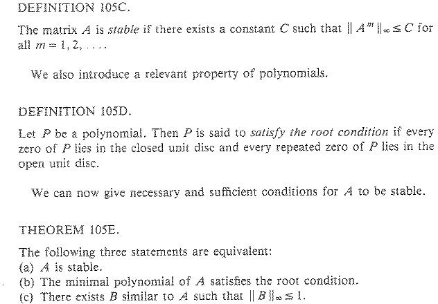
Let P be a polynomial. Then P is said to satisfy the root condition if every zero of P lies in the closed unit disc and every repeated zero of P lies in the open unit disc.
(Immediately following this statement is a theorem that a matrix A is stable (i.e. its powers are uniformly bounded) if and only if its minimal polynomial satisfies the root condition.)
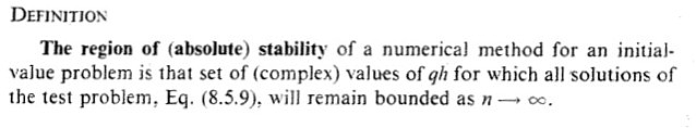
Definition: The region of (absolute) stability of a numerical method for an initial value problem is that set
of (complex) values of qh for which all solutions of the test problem y'=qy will remain bounded as n → ∞.
Definition 8.4 A multistep method is absoutely stable for those values ofλh where all of the roots of (8.17) are ≤1 in absolute value.
[Note that unless multiple roots of magnitude one are excluded, Gear's definition would allow solutions to grow algebraically. For this definition to make sense, this additional restriction is necessary. With that restriction, Gear's definition of the region of absolute stability equivalent to those of Butcher and Dahlquist.]
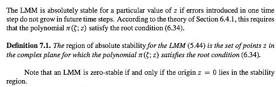
The LMM [linear multistep method] is absolutely stable for a particular value of z if errors introduced in one time step do not grow in future time steps. ... The region of absolute stability for the LMM (5.44) is the set of points z in the complex plane for which the polynomial π( ξ ; z) satisfies the root condition (6.34). Note that an LMM is zero-stable if and only if the origin z=0 lies in the stability region.
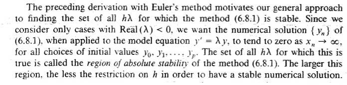
[ In case there is any doubt about the interpretation of the root condition, the previous page identifies the region of absolute stability of the leapfrog method as an interval on the imaginary axis, and describes the region of absolute stability of Euler's method with the condition |1+ λz| ≤1.
The region of absolute stability is the set of all h λ for which yn→ 0 as n → ∞
when the numerical method is applied to y' = λ y for all choices of initial values.
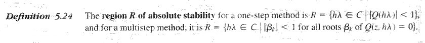
The region R of absolute stability for a one-step method is R = {hλ in C such that |Q(hλ)|<1},
and for a multistep method, it is R = {hλ in C such that βk<1 for all roots βk of Q(z,hλ)=0}.
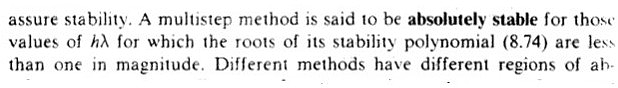
A multistep method is said to be absolutely stable for those values of hλ for which the roots of its stability polynomial (8.74) are less than one in magnitude.
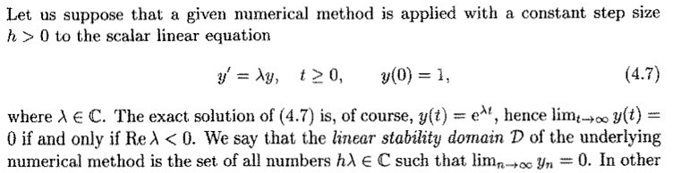
We say that the linear stability domain D of the underlying numerical
method is the set of all numbers hλ in C such that yn → 0 as n → ∞.
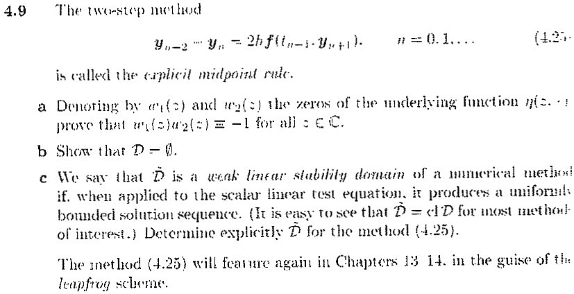
Iserles includes an exercise on p. 72 that defines a weak linear stability domain to deal with the emptiness of the linear stability domain of the leapfrog method. Iserles states that for most methods of interest, the weak linear stability domain is the closure of the linear stability domain. But that is clearly not the case for the leapfrog method of the exercise, since the closure of the empty set is the empty set, and the weak linear stability domain (our region of absolute stability) of the leapfrog method is the interval (-i,+i) on the imaginary axis. He even makes an off-the wall joke regarding the linear stability domain that had me literally laughing out loud when I got it. See the scanned page below.
Only the finest math books can make the reader laugh. Iserles' book meets this standard:
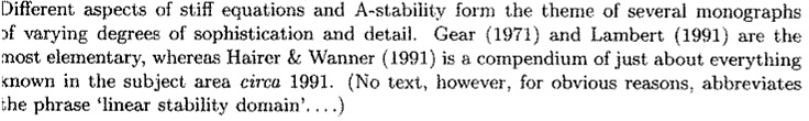
An exemplary book in so many ways! However, I couldn't resist contradicting his joke by abbreviating the phrase in ODE & CM, with a footnote to this page of Iserles.